GraphWeb overview
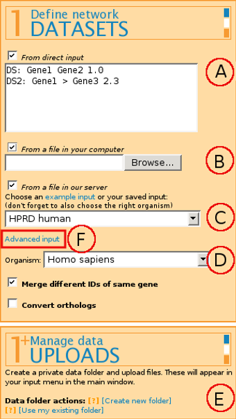
The format for input is:
Label: Gene_ID Gene_ID Weight
Label and Weight are optional parameters.
It is also possible to have directed edges by marking the directionality with < and > markings.
(B) From a file in your computer - allows uploading a file to the server for the current web browser session only. If you plan to use the same file next time as well, we suggest uploading the file to the server permanently by using (E) Manage data Uploads.
(C) From a file in our server - allows picking either a publicly available file from our example filelist or a file previously uploaded through (E) Manage data uploads (see below).
If you're working with biological data, select the correct Organism (D) for module scoring through g:Profiler that uses Gene Ontology, miRNA target genes, transcription factor binding sites and pathways.
Combining several input files is possible by "ticking" several or all of the input boxes mentioned above, or by using Advanced input (F).
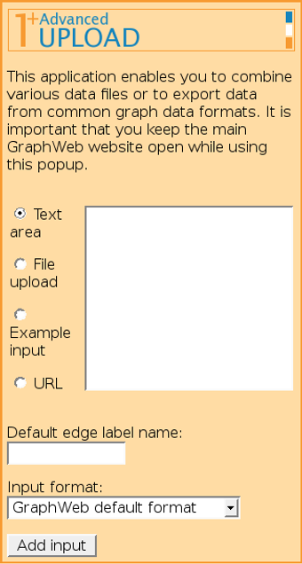
It is possible to add several input files (possibly from different origins) one by one and combine them into one network, possibly attaching different edge labels for data of different origin.

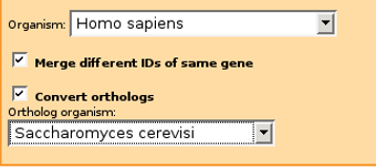
For example, if you have mainly human gene IDs originating from Ensembl and protein IDs from Intact databases, plus additional genes from yeast protein-protein interactions, you should pick Merge different IDs of same gene, Homo sapiens as Organism and also check Convert orthologs and select Saccharomyces cerevisiae as ortholog organism.
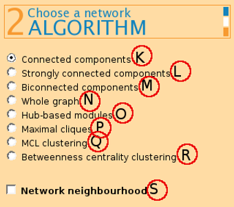
(K) Connected components - returns modules where a path exists between any two nodes.
(L) Strongly connected components - returns modules from a directed graph where a directed path from node u to v and vice versa exists between all pairs of nodes. On undirected graphs, this algorithm has the same effect as connected components.
(M) Biconnected components returns connected modules where a removal of any node does not disconnect the graph.
(N) Whole graph returns the graph as one module, after applying any network filters chosen by the user.
(P) Maximal cliques finds graphs of 4 or mode nodes where each node is connected to every other node.


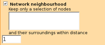
If the distance is set to 0 then only edges from selected dataset that connect user given nodes are found. It probably works best with the (K) Connected components algorithm.
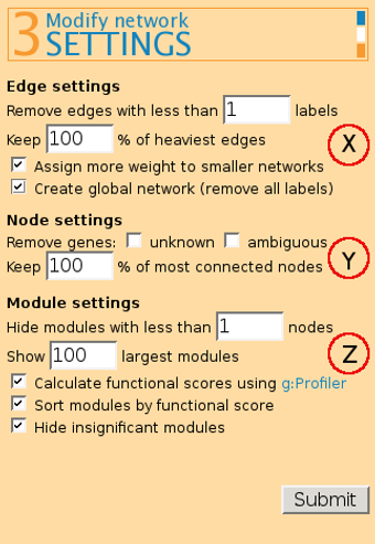
Remove edges with less than x labels. Edge labels are a method for distinguishing data from different sources that you might wish to combine. This feature allows testing which connections in the graph are supported by more data sources.
Keep x% of heaviest edges - removes edges by their weight, starting from lower scoring edges. Assign more weight to smaller networks - helps to automatically score small, better defined networks higher. The different networks should be specified by edge labels.
Create global network (remove all labels) - for merging all input networks together, if you don't want to see label information in the output while still keeping some of the benefits of labels (such as setting edge weights automatically).
(Y) Node settings:
Remove unknown and/or ambigous genes - allows user to remove genes that do not have any match in the main databases (unknown) or that have more than one match (ambiguous).
Keep x% of most connected nodes helps in removing nodes that have few neighbours (e.g. terminal child-nodes).
(Z) Module settings
Hide modules with less than x nodes - helps in filtering out modules that are too small and thus decreasing the output size.
Show x largest modules shows only the biggest modules, similarly to the previous option. It has been set to 100% by default.
Calculate functional scores using g:Profiler - gives a score for each module found by the algorithm, based on its biological significance. Only modules with size up to 1500 nodes are sent to g:Profiler and scored.
Sort modules by functional score - enables to order resulting modules in their putative functional importance.
Hide insignificant modules removes modules with score 0.

[b] Nodes is the number of nodes in current module.
[c] Edges expresses the number of edges in current module.
[d] Density score expresses the aspect ratio of edges in the module, compared to the greatest possible number of edges in a module with the given number of nodes.
[e] List nodes lists all nodes in the module.
[f] List edges lists all edges in the module.
[g] Zoom in links the module back to GraphWeb input. It is useful when one wants to split the current module further into smaller parts with a different algorithm or to apply filters to the current module.
[h] Label distribution contains a bar graph showing the distribution of labels between the edges of the module. Each color represents one dataset.
[i] Score characterizes the functional importance of the module. It is calculated using g:Profiler results. All p-values from statisticly significant terms are minus log-d and summed up and divided by the number of nodes in the network. Higher scores mean higher significance of the module. The cell is color-coded by 'higher score = redder cell'.
[j] Best g:Profiler results list the best term from each category that is used in g:Profiler. See below for more information.
[j] g:Profiler annotations links to g:Profiler for full annotations of the current module.
[k] Visualisations are graph layouts either with (labeled) or without (compact) gene names. Graphs bigger than X nodes are not visualized. It is also possible to see the graph layout in SVG format by clicking "" in pop-up window.
[m] Cytoscape input in SIF format. Useful for advanced visualizations and other type of network mining.
[n]g:Cocoa does comparative annotations of all modules from the output with GO, Reactome, KEGG, miRNA and TFBS.
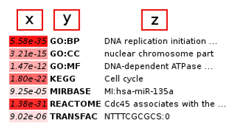
The best annotation from each category is output. The p-value is given in the first column [x], the subontology class in the second column [y] and the class description in the third column [z].
Color-coding (from white to red) is used for denoting more significant classes.
How are my favourite genes connected by protein-protein interactions (PPI)?
The Network neighbourhood feature is great for that.
(1) Paste gene IDs to the Network neighbourhood textarea (different ID types are supported).
(2) Set the distance parameter to 0.
(3) Select a file with PPI data from your computer or use data from our server (such as the 'Intact+HPRD+ID-SERVE human' dataset).
(4) Set the correct organism. [a] If your genes and PPI data are for the same organism then pick that organism from the menu. [b] If your genes are from one organism and the PPI data from another (e.g. genes from fly and PPI from human) then pick PPI data source organism from Organism menu and the other organism from Convert orthologs menu (e.g. 'Homo sapiens' from Organism and 'Drosophila melanogaster' from Convert orthologs).
Identify transcription factors with their common targets
The Biconnected components algorithm helps us out here.
(1) Upload a dataset containing TF - target gene pairs. (2) Select the Biconnected components algorithm.
(3) The algorithm identifies genes that are connected through two paths or more. If two transcription factors share at least 2 target genes, they will be in the same module.
Identify genes that play an important role (e.g. having many targets or being regulated by many genes in transcription network)
The Hubs-based modules algorithm finds genes that are connected to many other genes and displays them ordered by the number of neighbours.
(1) Select the dataset.
(2) Set Max distance from hub to 1 if you want star-shaped hubs, e.g. transcription factors and their direct targets. Set the parameter to 2 for also taking undirect targets into account. Be aware that the larger the distance parameter, the more time is needed for calculations.
(3) Make sure Sort modules by functional score is turned off, to sort modules by size.
(4) In the results, the name of the hub is shown in the first column along with the module number.
Find genes that coexpress and have protein-protein interactions.
Edge filtering can be used for extracting edges that have more than one label.
(1) Upload/or use from our server gene pairs from both gene expression and protein-protein interactions datasets. Do not forget to add different edge labels for the datasets. If you are using files from our server that don't have edge labels, use the Advanced input tool to add them (Default edge label name).
(2) Set x to 2 at Remove edges with less than x labels. In this way, only gene pairs that are connected in both datasets are used for module searching.
(3) Use whole graph to get the full network or to use other algorithms to find specific types of gene modules.
(1) Was the selected organism correct?
(2) The module size filter.
(3) The edge label filter.
(4) Uncheck the Network neighbourhood box if you don't want to use it.
(5) When using many datasets with different IDs, Merge different IDs of same gene should be checked.
Other questions:
(6) No visualisation given. Output module was too big to visualize with our method. You can use SIF output and visualize the module using Cytoscape.
(7) Module score is zero. Check if the organism was correct because the score is calculated by using g:Profiler.