 MEM - Multi Experiment Matrix help
Gene ID input
Gene IDs are converted using g:Convert (part of g:Profiler tool) which is built on Ensembl BioMart and thus supports all major gene identifiers, starting from Ensembl gene ID and converting it into platform specific probeset ID(s). In the case of multiple IDs, the user is required to select one. If the initial query is a valid probeset ID, it would be automatically selected.
Database selection
All experiments have been downloaded from the ArrayExpress database and the database of MEM is updated regularly to include all new datasets from ArrayExpress. For the sake of scientific consistency, all past updates are preserved as dated versions in the MEM database (Current always being the latest version; Publication denotes the state of the database at the time when the MEM interface article was published)
Collection selection
Experiments are divided into collections based on their microchip platform. The platforms appear in the list based on the number of experiments in the collection. Some of the platforms are marked with '*', this means we can not provide a nice way to map Affymetrix ID's on those platforms, since they are not yet present in Ensembl BioMart. The '*' will be removed once the platform is mapped trough BioMart!
Platforms can also be filtered by organism ID for more convenient usage.
Options
Similarity
Output
Gene filters
Dataset filters
 |
|
NetCDF output format explained
MEM allows to download results in NetCDF format. To successfully work with NetCDF files netcdf-bin, libnetcdf-dev and their dependencies should be present in the OS. The latter is required to install ncdf package in R. Example of mem NetCDF structure:
netcdf memcpp_res_8 .. 0 {
dimensions:
        focus = 100 ;                                     #number of datasets used in query
        nonfocus = 545 ;                                  #number of datasets left out due to filter (i.e. st-dev, etc)
        strlen_datasets = 64 ;                            #can be ignored / nr of characters reserved for dataset names /
        strlen_genes = 28 ;                               #can be ignored / nr of characters reserved for gene names /
        genes = 22282 ;                                   #number of features/probes/genes on platform
variables:
        char reference(strlen_genes) ;                    #query feature/probe/gene
        char focus_name(focus, strlen_datasets) ;         #dataset names for focus
        double focus_stdev(focus) ;                       #query feature/probe/gene-s st-dev for focus
        char nonfocus_name(nonfocus, strlen_datasets) ;   #not so interesting dataset names
        double nonfocus_stdev(nonfocus) ;                 #not so interesting st-dev values
        char gene_name(genes, strlen_genes) ;             #feature/probe/gene names for rest of the platform (i.e. not reference)
        double score(genes) ;                             #MEM similarity score for all genes (except reference)
        int support(genes) ;                              #number of datasets that contributed in score (boxed in matrix view)
        int score_rank(genes) ;                           #rank value at score
        int focus_rank(genes, focus) ;                    #rank matrix. Ranks for all features/probes/genes in every dataset
        int nonfocus_rank(genes, nonfocus) ;              #rank matrix for non-focus datasets
}
Depending of view options used, some NetCDF variables can be missing from above list, this does not mean it is broken. Use "Display all datasets .." from Output tab and try again.
Intro to R
Following code will open .nc file and read in two most important variables into R: named mem scores (w/o reference) and focus_ranks as rank matrix used to get mem scores.
library(ncdf)                                                   #load R NetCDF library
nc <- open.ncdf("memcpp_res_8 .. 0.nc")                         #open *.nc file / open.ncdf("<path/to/nc/file.nc>") /
  #read some variables from the file into R
reference <- get.var.ncdf(nc, "reference")                      #reference/query feature/probe/gene name
gene_names <- get.var.ncdf(nc,"gene_name")                      #feature/probe/gene names (except reference)
focus_ranks <- get.var.ncdf(nc,"focus_rank")                    #rank matrix (except reference)
scores <- get.var.ncdf(nc, "score")                             #mem scores (except reference)
names(scores) <- gene_names                                     #add names to scores array (w/o reference)

str(scores)       #mem scores with feature/probe/gene names (w/o reference)

ds_names <- get.var.ncdf(nc,"focus_name")                       #dataset names
ds_names <- sub(".*\\/","",sub(".nc","",ds_names), perl=T)      #make dataset names more comfortable
focus_ranks <- t(focus_ranks)                                   #transpose so that datasets would be in columns (not needed if only one dataset!)
focus_ranks <- rbind(rep(1,length(ds_names)), focus_ranks)      #add reference also to the rank matrix (has always rank 1, i.e. most similar to it self)
rownames(focus_ranks) <- c(reference,gene_names)                #define row names for the rank matrix
colnames(focus_ranks) <- ds_names                               #define column names for the rank matrix

str(focus_ranks) #focus rank matrix
If R is not the preferred analysis environment, then it is possible to convert NetCDF files to flat files with TabCDF
Word cloudsAbout the annotations:
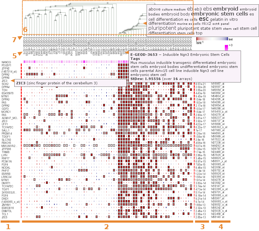
to every term in the datasets descriptions MetaMap tool was applied in order to annotate them. After that additionally to the basic word cloud out of the initial descriptions, the annotation word cloud was constructed. The significant terms that appear to have significant annotations in the annotation word cloud were replaced with their annotations. Additional terms from annotation word cloud that have not appeared in the basic word cloud were also added to the final word cloud.
One-way view
The word cloud consists of terms that are significantly most overrepresented across the datasets descriptions that contributed to the coexpression of the query gene with the selected gene. Since there is an ordering for the contributed datasets, the terms were tested to be overrepresented for ds_1; ds_1 and ds_2; etc. and the minimal out all these p-values was chosen as the final one for the term. Bonferroni correction was applied to these p-values due to the multiple comparisons issue. The word clouds were made more thorough by applying annotations to them using MetaMap tool.
Two-way view
The word cloud consists of terms that are significantly most overrepresented across the datasets descriptions that contributed to both coexpression of the query gene with the selected gene and vice versa. Since there is no ordering for the contributed datasets in this case, the terms were tested to be overrepresented only for the whole set of datasets simultaneously. The word clouds were made more thorough by applying annotations to them using MetaMap tool.